Basic MCMC Pt. 1: An Intro to Monte Carlo Methods

A common computation we face in machine learning is computing expectations. When working in \(\mathbb{R}^d\), for instance, we often face integrals of the form: \[\mathbb{E}_{X \sim p}[f(X)] = \int{f(x)p(x)dx}\] Sometimes we can compute these analytically (i.e. through the use of rules of integration). However, many such integrals we face in ML are such that providing an analytic solution is intractable or impossible. It is this exact situation that motivates Monte Carlo (MC) methods.

A Deterministic Approximation

Imagine we have some random variable X that is distributed according to a truncated exponential with a rate of 1. \[X \sim p(x)\text{ where } p(x) = \frac{1}Ze^{-x}, x\in[0,10] \] Z here is just a normalising constant to ensure that the support has measure 1 and the PDF integrates to 1. The density of X looks as follows:

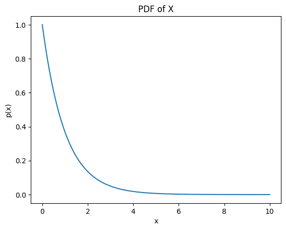
Now, say that we want the expected value of X. For reference, this is ~1 (or, to be precise, it is \(1-e^{10}=0.9999546\)). However, say that we cannot, for whatever reason, perform the below integral analytically. What do we do? \[I = \mathbb{E}_{X \sim p}[X] = \frac{1}Z\int_0^{10}{xe^{-x}dx}\]

One idea might be to try and use some numerical method to evaluate the integral deterministically. Basically, this means dividing the domain of integration up into blocks, approximating the value of the integrand for each block and summing these approximations. For instance, we might try dividing [0,10] up into unit-length intervals [0,1), [1,2) and so on, taking the value of \(xe^{-x}\) at the midpoint of each interval and then approximating the value of the whole integral as the sum of these midpoint approximations. Doing this yields an approximate value for the expectation of ~0.959. This seems like a pretty good guess for using such wide interval in our approximation, and we might think the best thing to do would just be to repeat this but using increasing narrow intervals.

This approach to evaluating integrals (roughly) corresponds to the idea of “Riemann discretization”. However, it leaves much to be desired. There are a few reasons for this:

The approximation we generate will be biased for any finite number of subdivisions of the domain of integration. This means any downstream use of the approximation will be incorrect in a systematic way.
As we have used a deterministic method, the nature of this bias is hard to characterise.
What happens when we are working in \(\mathbb{R}^d\) and d is large? We will need exponentially many subdivisions of the domain of integration to generate a reasonably accurate approximation. We can see this as an instance of the “curse of dimensionality”. Importantly, d often is huge in ML applications.

Monte Carlo Approximations

Importantly, the Monte Carlo approximation of an expectation overcomes all three of these shortcomings. An MC approximation works of the expected value of a distribution works as follows:

First, we sample N independent draws from the PDF p \[X_1\sim p(x_1),…X_N\sim p(x_n) \]
Then, we take generate our approximation the expected value, I, by summing them and dividing by N \[\hat{I}=\frac{1}N\sum_{n=1}^NX_n\]

Doing this for N=1000 (i.e. averaging over 1000 samples) for the above exponential example, we get an approximation of 0.975. This is very close to the true value!

More generally, if we wish to evaluate an expectation of the form \(I=\mathbb{E}_{X \sim p}[f(X)] = \int{f(x)p(x)dx}\), then the corresponding (vanilla) Monte Carlo estimator is defined as follows in \(\mathbb{R}^d\):

Suppose we can generate N independent and identically distributed (i.i.d) samples from the target measure p \[X_1\sim p(x_1),…X_N\sim p(x_n) \]
The, the vanilla MC is defined as: \[\hat{I}=\frac{1}N\sum_{n=1}^Nf(X_n)\]

Of course, this assumes that we can actually sample from the distribution of interest (which we rarely can in practice in Bayesian ML), but ignoring this we have a powerful estimator!

Importantly, as a function of random variables, the MC estimator \(\hat{I}\) is itself a random variabe. This means it has the properties of a random variable (such as a mean, a variance and a distribution) that allow us to characterise it. Importantly, it is therefore provably unbiased such that, unlike the deterministic approximation, it will not yield systematically wrong estimates. It is easy to show this: \[\mathbb{E}[\frac{1}N\sum_{n=1}^Nf(X_n)]=\frac{1}N\sum_{n=1}^N\mathbb{E}[f(X_n)]=\frac{N}N\mathbb{E}[f(X)]=\mathbb{E}[f(X)]\]

Additionally, unlike the deterministic method, Monte Carlo estimators are such that we can characterise their error by looking at their variance: \[Var(\hat{I})=Var(\frac{1}N\sum_{n=1}^Nf(X_n))=\frac{Var(f(X))}N\]

So, what does this all mean?

Well, as already stated it means that the estimator \(\hat{I}\) is an unbiased estimator of the expectation we seek to evaluate!
And, it doesn’t rely on some deterministic partition of the domain/support of the random variable like the Riemann discretization - this means we don’t suffer from the curse of dimensionality and can easily scale this method up to random variables living in higher dimensions!
Even better we can quantify the level of error expected in our approximation by considering the variance of the estimator around the true value of the expectation - this lets us be confident of better and better approximations as we increase the number of samples N and decrease the variance of the estimator!
Also, we can tell how “difficult” an expectation will be to approximate well (in terms of the number of samples we require to get a reasonably accurate approximation) since the variance of the estimator also depends on the variance of the function \(Var(f(X))\) under the sampling distribution. Hence, even if N is huge, if this variance is large we can tell a priori that our Monte Carlo approximation will leave much to be desired.
Finally, it can pretty easily be shown that this estimator obeys the Central Limit Theorem, and hence converges in distribution to the normal: \(\hat{I} \sim N(I, \frac{Var(f(X))}N)\)

Now, let’s see some of these properties in action for the truncated exponential example. First, let’s see that the MC approximation of the mean of this distribution improves as N increases. This is shown below, with the graph demonstrating the true value of the expectation (the dotted line) and the MC approximation for samples of different N:

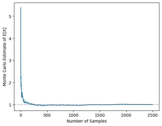
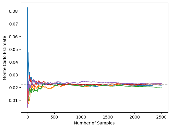
Clearly, as predicted by the fact that variance around the true value of the expectation decreases in N, as N increases, we get better and better approximations. We can see this “shrinking variance” effect by considering multiple different MC approximations. The graph below shows the MC approximations generated by 5 different, randomly-initialised MC approximations for different sample sizes:

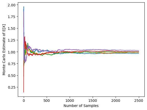
Clearly, as N decreases, we can see that the variance of these approximations decreases.

Problematic Functions

However, as mentioned above, some functions can be problematic in the sense that vanilla MC estimators struggle to converge to their true value for any reasonable finite value of N. This happens when the variance - or, “energy” - of the function under the sampling distribution is sufficiently high that increasing N doesn’t reduce the variance of the MC estimator.

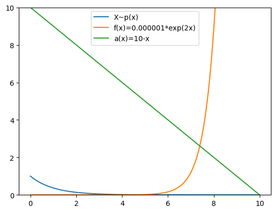
For instance, say we want to work out the expectation of \(f(x)=0.000001e^{2x}\) under our truncated exponential distribution. I have plotted both the function and the PDF of the distribution below - what do we see?

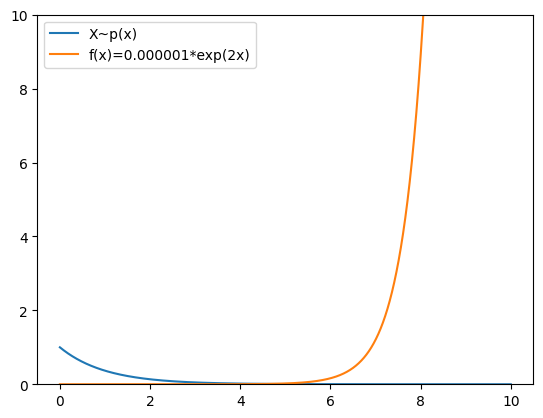
Well, what we see is that the region of high density under our distribution (which is the region in which most samples will be drawn) is on the left of the support while the important, non-zero region of f(x) is on the right. This means that the vast, vast majority of samples drawn from p will not contribute at all to the value of the expectation, and samples that do contribute to the value of the integral (e.g. samples that are near 10) will be exceedingly rare. In other words, the variance of the function under the distribution will be huge.

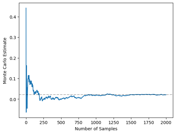
This means that the variance of the MC estimator will remain large even for large N, and will hence struggle to converge for reasonable sample sizes. This is illustrated in the graph below, where I plot the MC estimates for samples up to size 25,000 and we can see that the MC estimate still clearly hasn’t converged to the true value (dotted line).

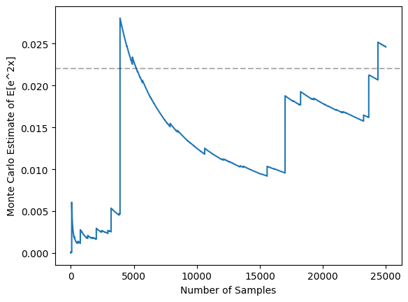
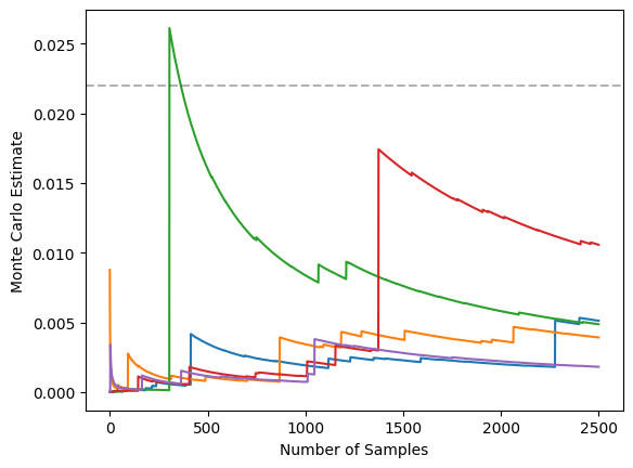
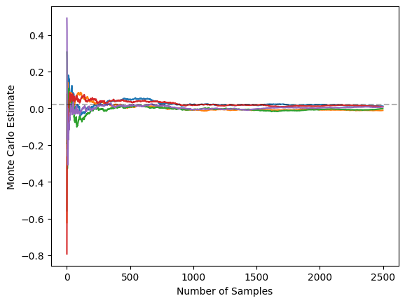
Indeed, this graph illustrate the problem well - most samples are nearly zero under f(x) (causing the estimate to decay toward zero most of the time), but very occasionally we get a sample near the right-hand side of the support that yields a huge value of f(x), causing the estimate to skyrocket. We can see that this causes high variance by considering 5 independent runs of MC estimates for this function:

So, what can we do when we want to take expectations of such functions?

Importance Sampling

One option we can take here is called importance sampling (IS). The idea of IS is, rather than sampling from p which is not in good alignment with f, to sample from some other distribution that is better aligned with f. In other words, we want to sample from some alternative distribution q that is more likely to produce samples from regions of the domain that are important for evaluating the expectation of f.

Now, if we can produce samples from q, we can use this to construct an IS Monte Carlo estimate of \(\mathbb{E}_{X \sim p}[f(X)]\) since:

\[\mathbb{E}_{X \sim p} [f(X)]=\int{f(x)p(x)dx}=\int{\frac{f(x)p(x)}{q(x)}q(x)dx} = \mathbb{E}_{X \sim q}[\frac{f(x)p(x)}{q(x)}]\]

Hence, we can define the IS Monte Carlo estimator as follows:

Suppose we want to estimate the expectation: \[I=\mathbb{E}_{X \sim p}[f(X)] = \int{f(x)p(x)dx}\]
Further, suppose we have some alternative probability measure q (called the “importance distribution”) such that \(q(x) \neq 0 \) whenever \(p(x) \neq 0 \) from which we can generate N i.i.d samples: \[X_1\sim q(x_1),…X_N\sim q(x_n) \]
Then, the IS MC estimator is defined as: \[\hat{I}_{IS}=\frac{1}N\sum_{n=1}^N\frac{f(X_n)p(X_n)}{q(X_n)}\]

Importantly, the previous line guarantees that this will be an unbiased estimator for the original expectation! Additionally, if we select a “good” q this estimator will have a significantly lower variance. A nice bit of intuition here for those that know some measure theory is that we are really just performing a change of probability measure by rescaling the integrand by the Raydon-Nikodym derivative of p with respect to q.

Now, it can be shown that the “optimal” (in the sense of maximally reducing variance) importance distribution q has a density given by: \[q(x) = \frac{|f(x)|p(x)}{\int{|f(x)|p(x)dx}}\]

I’m not including this proof to stop this post from getting too long, but proving this just requires showing that the new integrand’s variance has a lower bound (via Jensen’s inequality) and then showing that this lower bound is achieved if we choose q as our proposal distribution.

This optimal q makes a lot of intuitive sense - it says we want an importance distribution that assigns a high probability to samples being drawn from regions where both p(x) is high and f(x) is large in magnitude, since these are the regions that are important for evaluating expectations. Basically, if we use this optimal q we focus the samples we draw on important regions of the support and hence converge to the true value much faster.

In practice, this optimal q can be pretty annoying to find, and we can often just use a distribution that boradly meets this desiderata instead.

Now, let’s illustrate this with our truncated exponential distribution and the problematic f from above. Recall that the problem was that p placed most of its density on the left of the domain while the important regions for f where on the right. So, let’s try using an importance distribution that puts more density on the important regions of the domain. For instance, let’s set q to a trucated unit-scale Gaussian centered at 8: \[q(x)=N_{[0,10]}(x;8,1)\]

We can see why this is a broadly sensible q by considering f, p and q all on one graph and noticing the better alignement of q to the important region of the domain.

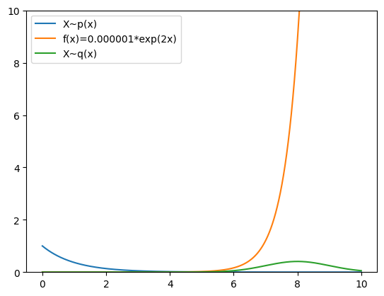
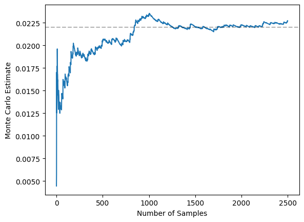
Given this better alignment, we expect faster convergence and reduced variance. This faster convergence is shown in the graph below, where we seem to have converged to the true value with 2,500 samples using the IS MC estimator. Recall that we hadn’t achieved this even within 25,000 samples for the vanilla MC estimator.

For reference, here is the analogous graph for said 25,000 samples with the vanilla MC estimator:

Additionally, this estimator has a much lower variance. The graph below illustrates this by showing 5 independent runs of the IS estimator

Again, for reference, here is the associated graph for 5 independent runs of the vanilla MC graph, clearly illustrating that IS has reduced variance massively:

In conclusion, importance sampling is pretty powerful and is fairly widely used, even in conjunction with more realistic methods (i.e. in MCMC contexts).

Control Variates

Another option for dealing with “problematic” functions in the context of basic Monte Carlo is to use control variates. The idea here is that we find some function f for which we know both its expectation under our distribution p and that its vanilla MC estimator is correlated with the vanilla MC estimator of our function of interest f. Then, we use this known correlation to “correct” our approximation of f. We do this since, for example, if the MC estimator of g is less than its known true value then the positive correlation with the MC estimator of f means f’s estimate will also be an under-estimate. Hence, it is sensible to “scale it up”.

More precisely, we define a control variate (CV) MC estimator as follows:

Suppose we want to estimate: \[I_f=\mathbb{E}_{X \sim p}[f(X)] = \int{f(x)p(x)dx}\]
Define the vanilla MC estimator \(\hat{I}_f\) as:

\[\hat{I}_f=\frac{1}N\sum_{n=1}^Nf(X_n)\]

Assume we have some function g for which we know the value of:

\[I_g=\mathbb{E}_{X \sim p}[g(X)] = \int{g(x)p(x)dx}\]

Further, define the associated vanilla MC estimator as \(\hat{I}_g\)

\[\hat{I}_g=\frac{1}N\sum_{n=1}^Ng(X_n)\]

Then, the control variate estimator of \(I_f\) is given by:

\[\hat{I}_{CV} = \hat{I}_f + \beta[\hat{I}_g - I_g]\]

So, why does this make sense as way of reducing the variance? Well, consider the variance of this new estimator:

\[Var(\hat{I}_{CV}) = Var(\hat{I}_f) + \beta^2Var(\hat{I}_g) + 2\beta Cov(\hat{I}_f,\hat{I}_g) \]

This is just a quadratic in \(\beta\). Minimising this gives the optimal \(\beta\) as:

\[\beta=-\frac{Cov(\hat{I}_f,\hat{I}_g)}{Var(\hat{I}_g)}\]

This formula makes sense - if the two estimators are positive correlated, the coefficient will be negative which corresponds to increasing the MC estimate of f whenever the mMC estimate of g is less than its true value. Plugging this back into the formula, we get a variance of the CV MC estimator of:

\[Var(\hat{I}_{CV}) = Var(\hat{I}_f) - \frac{Cov(\hat{I}_f,\hat{I}_g)^2}{Var(\hat{I}_g)} \]

Therefore, we get a reduction that is proportional to the covariance between \(\hat{I}_f\) and \(\hat{I}_g\)!

Let’s illustrate this with the truncated exponential and the problematic f again with \(g(x)=10-x\) as our control variate. To get a sense of the covariance between \(\hat{I}_f\) and \(\hat{I}_g\), I have plotted them (alongside p) on the graph below:

Now, this graphs tells us that \(\hat{I}_f\) and \(\hat{I}_g\) should be negatively correlated. This is because the “important regions” for f and g (or, the regions of f and g that take extreme values and hence contribute most to the expectation) are at opposite ends of the support of the distribution. For example, a sample that meaningfully increases \(\hat{I}_f\) will be a higher x value and hence will cause a proportionally smaller increase in \(\hat{I}_g\). This is all to say that samples that lead to over-estimates of the former MC estimator will be associated with under-estimates of the latter. Thus, we want to use a positive \(\beta\). Using \(\beta=0.5\), for example, yields rapid convergence within 2,000 samples as shown below:

Repeating the corresponding graph for 25,000 samples with the vanilla MC estimator again shows how this is a boost in performance:

And, using control variates yields a reduction in variance as shown in the figure below:

Repeating the corresponding graph for the vanilla MC estimator again shows how this is huge reduction in variance:

Summary

In summary, Monte Carlo methods are extremely powerful methods for calculating expectations that are either impossible or intractable to compute analytically. Additionally, techniques such as importance sampling and control variates allow us to use MC estimators even when we have problematic functions.

So, for the interested, why is understanding all of this so relevant to ML?

In much of ML we cannot fully specify distributions of interest and so cannot analytically calculate expectations with respect to them. Monte Carlo methods can be used to overcome this problem if we can still sample from the distributions.
Monte Carlo methods are combined with Markov chain methods in the suite of tools that are called “Markov Chain Monte Carlo” methods (MCMC). Markov chains allow us to sample from such distributions (even when we do not know their full explicit form), and we can then use Monte Carlo methods to marginalise out through the operation of taking expectations.
Such MCMC methods are very important in modern in machine learning. Diffusion models, for instance, are underpinned by theory relating to MCMC through the use of “Langevin dynamics”.
Finally, Monte Carlo methods are used heavily in modern RL due to the intractabality of analytically calculating the objective that we seek to maximise in RL. Control variates and importance sampling become very important when applying Monte Carlo methods to RL.