Exploring Tradeoffs Between Safety Metrics with MNIST

Despite huge advances in their capabilities when measured along standard performance dimensions (e.g. recognising images, producing language, forecasting weather patterns etc…), many deep learning models are still surprisingly “brittle”. While there are many dimensions along which this “brittle-ness” shows itself, three interesting ones are:

1. some models are surprisingly non-robust to inputs perturbed in specific, minimal ways not seen during training
2. some models are frequently unable to tell when an input is out-of-distribution or unlike other inputs it has seen
3. some models are still poorly calibrated, in the sense that their internal representations of uncertainty do not accurately reflect reality

In this post I will outline these issues - which we can view as being dimensions along which a model can be “safe” - with respect to a simple classifier trained on MNIST in the context of a project I did a while back. In retrospect, I think the project left a lot to be desired (I’ll get into this in the empirical section below), but I still think writing up this summary is worth it. For one, this was the first ever ML project that I did and I am definitely nostalgic about it since it kinda set me on the path I am on now. Additionally, I still think the topic (of empirical “AI safety” in the broad sense) is absolutely fascinating.

1 - Background

1.1 - Model Robustness

One ways in which models can be “brittle” is that they can suffer from a lack of robustness to minor changes in inputs. In the context of an image classifier, this lack of robustness exhibits itself as models being unable to accurately classify images that have undergone pertubations that are irrelavant / unnoticable to humans but that cause the model to fail.

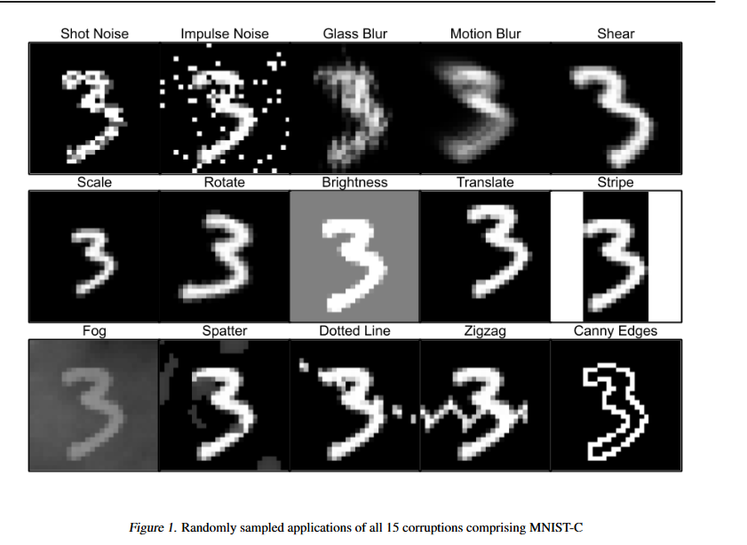
One kind of such image are distribution-shifted images. We can roughly see these as being images that, to a human, seem just as easy to classify as the images the model was trained on, but that have some visual effect - like snow or jitter - applied to them. Thus, we can think of them as being images drawn from a different distribution to the training examples, but from a distribution that seems qualitatively similar enough that the broad semantics remain unchanged and so model performance should transfer fairly well.

For example, the following are some distortions from the MNIST-C dataset (Mu and Gilmer, 2019; figure 1 from their paper). In all of these cases, despite looking like an easy “3” to classify, baseline MNIST classifiers often struggle hugely.

Another kind of image that image classifiers are often non-robust to are adversarially distorted images. These are images that an “adversary” has distorted in such a way as to make it hard for a model to classify accurately.

A common type of adversarial attack is a gradient-based adversarial attack. The basic idea here is that an adversary works out the gradient of the loss with respect to each pixel in an image and then takes mini steps in the direction that increases loss. There are many types of gradient-based attacks but I will just consider two popular variants.

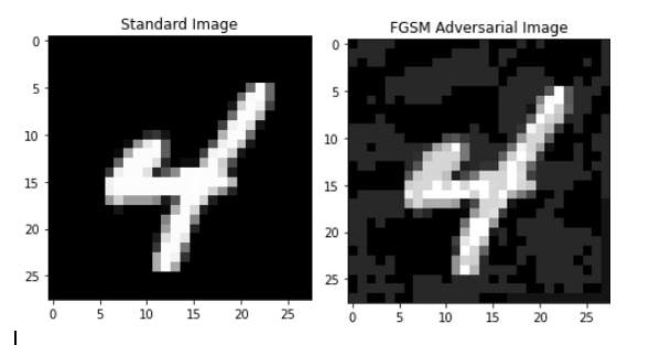
The first attack is the Fast Sign Gradient Method (FGSM) as introduced in (Goodfellow, Schlens, and Szegedy 2014). If \(x\) is an image, \(y\) is its label and \(l(x, y)\) is the loss associated with the model for whatever the model predicts for this image, then the FGSM-attacked image is given by: \[x_{FGSM}=x+\varepsilon \times sign(\nabla_xl(x, y))\]

Thus, FGSM distorts each pixel by an amount \(\varepsilon\) (which we call the “attack budget” and is a hyperparameter set by the user) in a direction that increases model loss. This ensures that the \(l_{\infty}\) norm of the distortion is trivially bounded by \(\varepsilon\). Basically, FGSM just performs a single bounded step of gradient ascent. In practice, this results in images that seem very similar to the human eye but that models struggle to classify accurately. The below example illustrates a 4 from the MNIST data before and after an FGSM adversarial attack is applied:

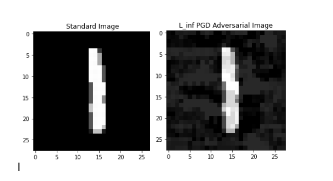
The second kind of adversarial attack I considered was projected gradient descent (PGD), which we can kind of think of as being a more powerful form of FGSM. PGD is very similar to FGSM except that it performs many small steps of gradient ascent rather than one big one as FGSM does. The broad steps of a PGD attack with an attack budget of \(\varepsilon\) and step count of \(N\) are as follows:

• First, randomly jitter the image \(x\) \[x_{PGD}=x+\eta, \eta \sim U[-\varepsilon, \varepsilon]\]
• Then, for \(t=1,…,N\), perform a step of gradient ascent to distort each pixel in a direction that increases loss \[x_{PGD}=x_{PGD} + \beta \times sign(\nabla_{\delta}l(x_{PGD}+\delta, y))\]
• After each step, if the \(l_{\infty}\) norm of the total distortion exceeds the attack budget, clip the distortion back into the \(l_{\infty}\) ball of size \(\varepsilon\) around the original image

So, this PGD attack performs multiple steps of gradient ascent to find a distortion that remains in a \(\varepsilon\)-ball (in terms of \(l_{\infty}\) norm) around the original image (though we can equally well use PGD with other norms). Thus, PGD can be seen as trying to find a “better” distortion than FGSM while remaining within the same attack budget. An example where I have applied PGD to an MNIST digit is shown below:

1.2 - Detecting Out-Of-Distribution Inputs

Alongside robustness, another dimension along which a model can be “safe” is its ability to recognise out-of-distribution (OOD), or, anomalous, inputs. The idea here is that we want a model to realise when it is fed an input that is radically different from other inputs it has seen. This will become an increasingly important consideration as models are deployed in more and more sensitive real-world applications.

The most common kind of technique for endowing models with the ability to detect anomalies involves anomaly scoring. Anomaly scoring techniques extract from models an “anomaly score” for each input, classifying that input as an anomaly if the score crosses some threshold. A common scoring technique involve using of maximum softmax or logit values for an input (Hendrycks and Gimpel 2017).

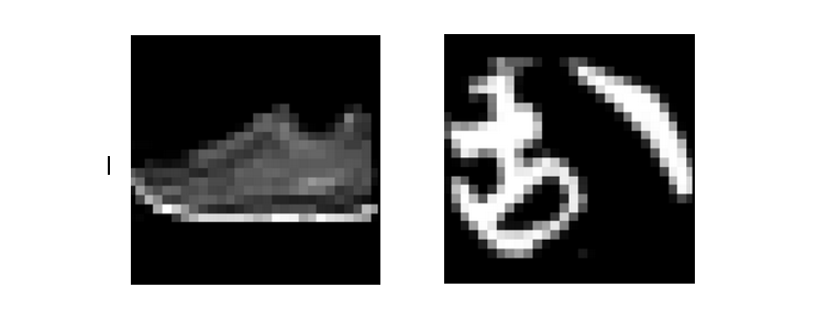
Two examples of inputs that we might want an MNIST classifier to flag as OOD are shown below. The examples are, respectively, from the F-MNIST dataset (Xiao, Rasul, and Vollgraf 2017) and K-MNIST dataset (Clanuwat et al. 2018)

1.3 - Calibration

The final dimension of model safety I considered was calibration. The idea here is that we want models to be able to quantify how certain / uncertain they are in their outputs since there is a lot of difference between an output that a model is 50.1% confident in as opposed to one it is 99.9% confident in. As such, we want to train our models not just to be accurate, but also to be well calibrated such that, for instance, when it makes a prediction with 60% confidence, it will be correct in that prediction 60% of the time

1.4 - Techniques for Improving Safety

I considered two commonly-proposed general techniques for improving model safety along the outlined dimensions. The first of these is the use of data augmentation during the training process, while the second is architectural changes.

Many commonly-proposed solutions to our safety issues involve using specific techniques to augment the data on which a model is trained on in some way. There are, broadly, two rough categories of such techniques.

The first of these is adversarial training (Madry et al. 2017), in which a certain portion of the data on which a model is trained on is adversarially distorted using some adversarial attack method. The hope here is that such adversarially distorted training data can act as a sort of regulariser. I only considered PGD and FGSM adversarial training, although other types do exist and this is something I would definitely change if I re-did this work.

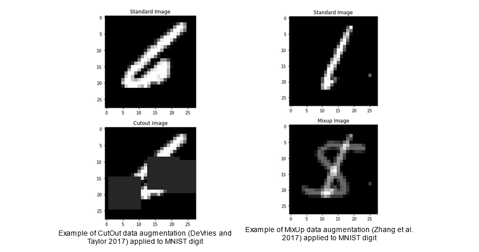
The second category of such techniques involves augmenting the training data in non-adversarial ways but similarly aiming to mimic regularisation. Many such techniques exist, but I focused on the data augmentation techniques of CutOut (DeVries and Taylor 2017) and MixUp (Zhang et al. 2017). In CutOut, a specified number of squares of specified size are “cut out” of the image in order to hide certain parts of the image from the model, and encourage the learning of more robust features (DeVries and Taylor 2017). In MixUp, input images are combined in a convex way such that the label which the model ought to assign to them is the respective convex combination of labels (Zhang et al. 2017). Both of the data augmentation techniques are illustrated below.

The final category of techniques I consider in this report are modifications to models that we could group under the label of “architectural”. The first of these modifications I consider is model size, since larger models are frequently found to perform better with regards to many safety metrics (Hendrycks et al. 2021). The second of these modifications I consider is model ensembling. Model ensembling involves combining the outputs of many separately trained models in order to produce a final output

2 - Methodology

2.1 - Model Implementations

The baseline model I used for comparison was the modification of the standard Le-Net 5 that is frequently used to illustrate the power of convolutional networks on the MNIST digit recognition problem. As expected, this model achieves a high accuracy rate (0.993) on the standard MNIST problems. I modified this network with various forms of the above techniques for improving safety.

2.2 - Safety Metrics

To benchmark robustness to adversarial attacks, I used as a metric the accuracy of each model in the face of the PGD and FGSM adversarial attacks over different attack budgets.

To benchmark robustness To benchmark robustness to distribution shift, I measure model accuracy on the MNIST-C dataset I discussed above.

To explore the ability of models to detect OOD inputs in our MNIST case, I used the F-MNIST and K-MNIST datasets as examples of OOD inputs that our MNIST classifier ought to recognise as OOD. I then tested the ability of different methods to successfully detect OOD inputs, using the AUROC scores as a metric for success.

To test calibration, I tracked the expected calibration error, RMS calibration error and brier score for each model on the original MNIST dataset. These metrics are all different measures of the same underlying concept, which is the ability of models to make well calibrated predictions such that an event X will happen 60% of the time when the models predict X with a confidence of 0.6

3 - Results

3.1 - Adversarial Robustness

The first area I explored was adversarial robustness, which I measured using the accuracy of models in the face of adversarial attacks of increasing strength. An interesting pattern emerges here. Across all models and all attack budgets, there appears to be three qualitatively different types of models. The figures below, which outline the adversarial accuracy for all models across all attack budgets with select models labelled, illustrates this pattern.

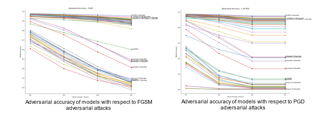
The pattern that is illustrated in these figures is that all the models tested fall into one of three categories.

First, we have a set of models that perform consistently worse than all other models. This set consists of the baseline model, and all models trained purely using those data augmentation techniques that aim to improve OOD robustness (e.g. Cutout and Mixup). Indeed, further inspection of this set of models reveals that the models trained using these OOD robustness enhancing techniques actually perform worse with regard to adversarial robustness than the baseline model. One interesting point here is that CutOut seems to be the superior data augmentation technique of the two from the point of view of adversarial robustness since it results in less of a decline in accuracy relative to the baseline.

The next overall set of models is the set of models that consistently achieve high accuracy in the face of both attacks across a range of attack budgets. This set consists of three types of models. It consists of those models that were trained solely using adversarial training, with FGSM and PGD adversarial training achieving similar results. It also contains models trained with both adversarial training and augmented training examples.

The finally qualitatively distinct set of models is those models that outperform the baseline models and augmentation models, and yet underperform the models trained using some form of adversarial training. This set consists of ensemble models, and the large version of the baseline model.

3.2 - Out-Of-Distribution Robustness

The idea that there is a tradeoff between adversarial robustness and OOD robustness is, somewhat at least, supported by the experiments I performed regarding the robustness of models to distribution shift.

From a high-level perspective, two conclusions arise when considering robustness to distribution shift. Firstly, many models follow a similar pattern such that they all suffer precipitous declines in accuracy when faced with the fog and impulse noise distortions. Secondly, while most models seem to follow similar overall patterns, there is much variability in accuracy with regard to each individual distortion.

The pattern with respect to ensembles remains similar to, albeit less pronounced than, with adversarial robustness. Specifically, all ensemble models slightly outperform the baseline model, with large ensembles doing better. However, the pattern for larger models is reversed, with larger models being less robust to distribution-shifted inputs. This provides mixed evidence for the hypothesis that there is a tradeoff between adversarial and OOD robustness. On one hand, larger models seem to improve adversarial robustness whilst hurting OOD robustness, while on the other large ensembles seem to improve both.

However, more evidence in favour of the tradeoff hypothesis comes from inspection of the data regarding adversarially trained models. All models trained purely with adversarial training (which happened to be the best performing models in terms of adversarial robustness) are less accurate on average over the OOD MNIST-C dataset. Another point of interest here is that those models that were adversarially trained with a stronger attack budget (which happened to be the most adversarially robust) have, on average, lower OOD robustness than those models trained with a smaller attack budget. Finally, it should be noted that adversarial training actually seems to improve model accuracy with respect to a specific distortions. This is perhaps interesting as it points towards adversarial training encouraging the learning of specific representations that are helpful in some contexts but harmful in others

Finally, we can turn attention to models trained using both data augmentation and adversarial training. I found little evidence that the order of the two processes made much difference in terms of OOD robustness.

3.3 - Anomaly Detection

As previously discussed, another important “safety” property that ML models can have is the ability to detect inputs that are anomalous compared to their training data. We can measure the ability of models to do this by providing them with a dataset consisting of both examples similar to those they were trained on and examples representing a distribution shift relative to those they were trained on, and then tracking their ability to use whatever anomaly scoring method we decide on to successfully detect the anomalous examples. We track this using the AUROC, where an AUROC of 1 corresponds to perfect classification of anomalous inputs, and an AUROC of 0.5 represents random chance.

Some of the key results here are as follows. Firstly, all models achieve relatively high AUROCs on both datasets, with most models achieving AUROCs of at least 0.90 across all datasets.

Turning our attention to specific families of models, more definitive conclusions arise. Let’s first consider ensemble models and the large version of our baseline model. A notable finding is that all ensemble models achieve higher AUROCs than the baseline model, with the improvement seeming to grow as the size of the ensemble increases. This is notable since this is the same pattern that emerges when considering both adversarial robustness and OOD robustness, implying that we can increase model safety metrics without incurring tradeoffs by using model ensembles.

However, this finding does not replicate for the larger version of the baseline model. Whilst this large model achieves a somewhat comparable AUROC for the K-MNIST data, it significantly underperforms the baseline model for F-MNIST. As such, given the improvements to adversarial robustness from this larger model, larger models seem to increase robustness at the cost of reducing their ability to detect anomalies.

Shifting focus to purely adversarially trained models, few conclusions seem to arise. For models adversarially trained using both PGD and using FGSM, no consistent pattern in AUROCs seems to arise and the overall effect remains ambiguous. In both cases, all models seem to achieve roughly comparable AUROCs as the baseline model.

More interesting findings emerge when we consider the performance of models trained using data augmentations. Specifically, I found that models trained using Mixup were notably less able to detect OOD examples than the baseline model, implying a tradeoff between OOD robustness and anomaly detection.

However, I found that the opposite was true for all models trained using some form of cutout. Specifically, I found that models trained using Cutout (either in isolation, or combined with some form of adversarial distortion) were significantly better at detecting anomalous inputs than the baseline mode, scoring higher AUROCs

3.4 - Calibration

Finally, we can turn attention to the performance of the different families of models with regards to calibration. Like with adversarial robustness, there are again three broad tiers of models.

The first tier is the worst overall tier that scores notably higher than the other models (including the baseline) on all calibration metrics. Interestingly, this tier of models consists solely of those models that were trained by first applying Mixup and then applying adversarial training. This is a notable finding, since it is the only case (other than that of ensemble models) where models of a single type are in a category of their own.

Skipping a tier, the third and best tier of models consists of ensemble models. Ensemble models achieve better results than all other models and significantly outperform the baseline model. Additionally, the larger the size of the ensemble model, the better calibrated it is

Finally, the middle tier of models consist of all other models I considered, with pretty much all of them achieving worse calibration results than the baseline. This includes all models trained using adversarial attacks, data augmentations and any mix of the two except mixup followed by adversarial distortions

4 - Conclusion

Having considered all of the above experiments, we can finally return to the question of whether or not there are tradeoffs between different safety metrics that it might be desirable for a model to have. I would contend that the experiments conducted here are mixed in their answer to this question.

On one hand, they imply that yes, we can achieve good performance on all these safety metrics if we use ensemble models. This is because ensemble models outperformed the baseline model with regard to all four of the safety properties tested here (adversarial robustness, OOD robustness, anomaly detection and calibration).

However, this affirmative response must be qualified. This is because ensemble models do not always achieve the highest performance on any single calibration metric, and those models that do achieve this best-in-class performance on any single safety metric often end up underperforming the baseline model on another metric. For instance, the models that achieved the best adversarial robustness were those models that were trained using some form of adversarial training. For example, many adversarially trained models outperformed all ensemble models by >50% in terms of adversarial accuracy, yet end up being incomparably worse when it comes to OOD robustness. As such, in the sense of achieving the best result possible on any single metric, it does appear that there is sometimes a tradeoff

5 - Reflections on these Experiments

Looking back, there’s a lot in this work I am not happy with. A few key things that stand out are:

• I trained models on the same adversarial attacks as I tested their adversarial robustness using - this goes in the face of work that has found that robustness to one type of attack does not guarantee robustness to others
• I only considered very weak adversarial attacks - the literature has advanced considerably since PGD and FGSM came out, and much more powerful variants now exist
• All experiments were done with MNIST - some work has found that robustness on MNIST doesn’t correlate with robustness on other datasets due to its almost “toy” nature

At some point I’d like to re-do this kind of research on something like ImageNet with an eye to the current state of the literature. This is because not only do I think this topic is really interesting, but I also think this “pragmatic view of AI safety” will become increasingly important as ML models are embedded in the world around us in the future.

References

The following is a full list of reference I cited in the report that might be of varying degrees of interest:

Borowski, Judy, Roland S. Zimmermann, Judith Schepers, Robert Geirhos, Thomas S. Wallis, Matthias Bethge, and Wieland Brendel. 2021. “Exemplary Natural Images Explain CNN Activations Better than State-of-the-Art Feature Visualization.”

Bostrom, Nick. 2014. Superintelligence: Paths, Dangers, Strategies. Oxford: Oxford University Press.

Clanuwat, Tarin, Mikel Bober-Irizar, Asanobu Kitamoto, Alex Lamb, Kazauki Yamamoto, and David Ha. 2018. “Deep Learning for Classical Japanese Literature.”

Cunn, Yann L., Leom Bottou, Yoshua Bengio, and Patrick Haffner. 1998. “Gradient-Based Learning Applied to Document Recognition.” PROCEEDINGS OF THE IEEE.

Deng, Li. 2012. “The mnist database of handwritten digit images for machine learning research.”

DeVries, Terrance, and Graham W. Taylor. 2017. “Improved Regularisation of Convolutional Neural Networks with Cutout.”

Goodfellow, Ian J., Jonathon Schlens, and Christian Szegedy. 2014. “Explaining and Harnessing Adversarial Examples.”

Hendrycks, Dan, Steve Basart, Norman Mu, Saurav Kadavath, Frank Wang, Evan Dorundo, Rahul Desai, et al. 2021. “The Many Faces of Robustness: A Critical Analysis of Out-of-Distribution Generalization.”

Hendrycks, Dan, Nicolas Carlini, John Schulman, and Jacob Steinhardt. 2022. “Unsolved Problems in ML Safety.”

Hendrycks, Dan, and Kevin Gimpel. 2017. “A Baseline for Detecting Misclassified and Out-of-Distribution Examples in Neural Networks.” ICLR 2017.

Hendrycks, Dan, Mantas Mazeika, and Thomas Dietterreich. 2018. “Deep Anomaly Detection with Outlier Exposure.” ICLR 2019.

Kingma, Diederik P., and Jimmy L. Ba. 2015. “Adam: A Method for Stochastic Optimization.” ICLR 2015.

Lipton, Zachary. 2016. “The Mythos of Model Interpretability.” 2016 ICML Workshop on Human Interpretability in Machine Learning.

Madry, Aleksander, Aleksander Makelov, Ludwig Schmidt, Dimitris Tsipras, and Adrian Vladu. 2017. “Towards Deep Learning Models Resistant to Adversarial Attacks.”

Mu, Norman, and Justin Gilmer. 2019. “MNIST-C: A Robustness Benchmark for Computer Vision.”

Olah, Chris, Alexander Mordvintsev, and Ludwig Schubert. 2017. “Feature Visualization.”

Ovadia, Yaniv, Emily Fertig, Jie Ren, Zachary Nado, D. Sculley, Sebastian Nowozin, Joshua Dillon, Balaji Lakshminarayanan, and Jasper Snoek. 2019. “Can You Trust Your Model’s Uncertainty? Evaluating Predictive Uncertainty Under Dataset Shift.” 33rd Conference on Neural Information Processing Systems (NeurIPS 2019).

Russel, Stuart. 2019. Human Compatible: Artificial Intelligence and the Problem of Control. N.p.: Viking.

Schott, Luks, Jonas Rauber, Mathias Bethge, and Wieland Brendel. 2018. “Towards the first adversarially robust neural network model on MNIST.”

Strauss, Thilo, Markus Hanselmann, Andrej Junginger, and Holger Ulmer. 2018. “Ensemble Methods as a Defence to Adversarial Perturbations Against Deep Neural Networks.”

Wang, Haoqi, Zhizhong Li, Litong Feng, and Wayne Zhang. 2022. “ViM: Out-Of-Distribution with Virtual-logit Matching.”

Xiao, Han, Kashif Rasul, and Roland Vollgraf. 2017. “Fashion-MNIST: a Novel Image Dataset for Benchmarking Machine Learning Algorithms.”

Yun, Sangdoo, Dongyoon Han, Seong J. Ooh, Sanghyuk Chun, Junsuk Choe, and Youngjoon Yoo. 2019. “CutMix: Regularization Strategy to Train Strong Classifiers with Localizable Features.”

Zhang, Hongyi, Moustapha Cisse, Yann Dauphin, and David Lopez-Paz. 2017. “Mixup: Beyond Empirical Risk Minimisation.”