Variational Dropout in Recurrent Models

A workhorse of deep learning is dropout which is typically thought to help limit the extent to which models overfit to training data. However, the question of how to apply dropout to recurrent models that process inputs sequentially lacks a trivial answer. In this blog post, I will explore the problem of applying dropout to recurrent models and outline the idea of “variational dropout” as introduced in Gal & Ghahramani (2015). As such, this post is more or less a shoddy re-explanation of that paper, so the interested reader is encouraged to go read that. I have also implemented this as part of my BadTorch project which I will probably write about at some point soon.

Dropout

A key capability that we wish for models to acquire is the ability to generalise from inputs they have learnt to correctly handle training to unseen inputs they encounter “out in the wild” when deployed. Generalisation requires training models on training datasets in such a way that they learn the generalisable patterns inherent to the data without fitting to the noise specific to the training data. This problem of fitting to the noise in the data is the so-called problem of overfitting.

A common technique for encouraging models to avoid overfitting to the data is dropout. I assume the reader is somewhat familiar with dropout since it is pretty ubiquitous but will give a brief overview now in case this is not the case.

Dropout, as introduced in Srivastava et al. (2014), is motivated by the idea that overfitting can arise when individual hidden units in a model co-adapt to specific quirks of the training data. The worry here is that, if we train a model for an overly long time on some training data, we may end up minimising loss be encouraging many hidden units to work together to represent noise in the training data that is unnrelated to the patterns we wish for it to learn. This is because the models will be able to better predict training labels by, effectively, memorising the training data rather than trying to infer the underlying pattern that explains the link between training examples and their labels.

To avoid this from happening, Dropout “drops” hidden units at random while training. What this means is that whenever we pass a batch of training data through the model, we randomly set some hidden units to be zero before passing on to the next layer. A nice visual illustration of this is the below figure taken from the afforementioned original dropout paper.

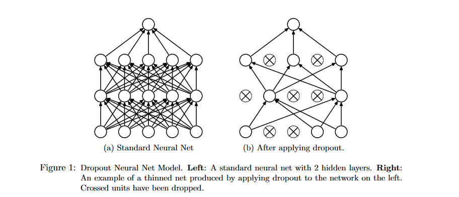
The idea here is that, by randomly “turning off” hidden units during training, hidden units cannot collectively learn to represent quirks of the training data since units can never depend on other units being present.

More specifically, we choose a dropout strength \(p \in [0,1]\) and, with independent probabilities \(p\), randomly set each individal hidden unit to zero. In other words, dropout introduces a \(Bernoulli(p)\) random variable for each hidden unit that masks out that hidden unit when it is turned on (which, of course, happens with independent probability \(p\)).

Now, since we are randomly zeroing out hidden units during training, the obvious question to ask is what do we do at test time? One option is to view dropout in Bayesian terms (more on this below) such that the dropout masks applied at each training pass correspond to drawing a sample of network weights from a distribution (since zeroing out hidden units leads to the corresponding weights not contributing to predictions). Then, we can provide a Monte Carlo approximation of the expected output of the model by running the model multiple times on each input and averaging the outputs. While nice in terms of its theoretical justification, this technique is not that popular in practice. Instead, people tend to multiply all weights by \(1-p\) at test time, with the thought being here that this corresponds fixing to the expected value of the hidden unit times any weight.

The type of dropout described above is what is commonly meant when dropout is referred to in deep learning and has been found to be massively succesfull at preventing overfitting such that models can spend longer learning generalisable patterns in training data. As such, dropout is a form of regularisation. For the rest of this post, I shall refer to this of dropout that randomly masks out hidden units whenever data is passed through as being “standard dropout”.

Applying Dropout To Recurrent Models

We can then turn attention to regularising recurrent models like GRUs and LSTMS. While such recurrent models are maybe less popular than they were a few years ago given the advent of transformers, this is, I think, still a pretty interesting topic for two reasons:

• First, it relates to the broad question of generalisation in deep learning which is both hugely important and still lacking a completely solid theory. Investigating generalisation in the context of recurrent models is then of interest since it helps build a vague sense of intuition about how this kind of thing ends up working in practice.
• Second, while recurrent models aren’t quite as powerful as transformers given unlimited access to compute, I have personally found them to be better given limited compute.

Whether or not standard dropout would be able to succesfully regularise a recurrent model is an interesting question. This is because, in a recurrent model like an LSTM, we pass each element in an input sequence through a model sequentially. Thus, standard dropout would involve applying a new dropout mask to the hidden units at each step of the sequence. Now, this intuitively seems like it might be a cause for concern since it conceptually leads to a different form of regularisation than when standard dropout is applied to a non-recurrent model. This is since we are now applying many different dropout masks over the course of a single forward pass of training. Thus, the gradient updates that will be being performed on the backward pass will lead to intuitively different kinds of updates as we will be backpropogating through combinations of multiple different dropout masks at once.

Why might this be as problem? Well, intuitively, it means we are effectively adding more noise into the network at each step of the input sequence rather than just adding one injection of noise as with dropout in non-recurrent models. Hence, while the noise in standard dropout as applied to non-recurrent models is helpful for regularising, we might worry that standard dropout would inject sufficiently loud noise into a recurrent model that the model would no longer be able to infer the patterns hidden in the data through it. This then motivates the question of how to apply dropout to regularise a recurrent model.

A Brief Overview of Bayesian Neural Networks

Before turning to a proposed solution to this problem, it is useful to first very briefly overview Bayesian neural networks. The core idea here is that we want to somehow approximate the predictive distribution \(p(y^*|x^*, X, Y)\) over the label \(y^*\) for some unseen input \(x^*\) given our training data \((X, Y)\). For classification tasks like those being considered here, this predictive distribution will be a distribution over the labels. If we call the parameters of a network \(\omega\), we can do this by introducing a posterior \( p(\omega|X, Y) \) over these parameters and then marginalising them out:

\[p(y^*|x^*, X, Y)=\int{p(y^*|x^*, \omega)p(\omega|X, Y)d\omega}\]

We often then place a standard Gaussian prior over the weights of the network and the likelihood \(p(y^*|x^*, \omega)\) is just the distribution over class labels for the given parameters \(\omega\).

But, what actually is the posterior over network parameters? Well, as is the case a lot of the time in Bayesian statistics, this kind of distribution ends up being analytically intractable. However, we can approximate it using variational inference.

An Even Briefer Overview of Variational Inference

What, then, is variational inference? The general idea here is that there is some distribution \(p(x)\) that is of interest but that is unknown. Variational inference then involves introducing some known distribution \(q(x)\) - called the “variational distribution” and then minimising the KL divergence (which measures how “far apart” two distributions are in an abstract sense) between the variational distribution and the distribution of interest. The resulting variational distribution then ought to be a good approximation to the original, unknown distribution.

We can then use variational inference to find a variational approximation \(q(\omega)\) to the posterior over the network weights \( p(\omega|X, Y) \). If we are predicting class labels from a set of K possible labels, this KL divergence then looks like:

\[KL(q(\omega)||p(\omega|X, Y)) \propto - \int{q(\omega)log(p(Y|X, \omega))d\omega} + KL(q(\omega)||p(\omega)) \]

where \(p(\omega)\) is our prior over the network parameters. Now, say we have N training examples in the training dataset \((x_i, y_i)\) and let the logits produced by our model for the i-th training sequence when our parameters are \(\omega\) be denoted \(f^\omega(x_i)\). We can then decompose the KL further as:

\[KL(q(\omega)||p(\omega|X, Y)) \propto - \sum_{i=1}^N\int{q(\omega)log(p(y_i|f^\omega(x_i)))d\omega} + KL(q(\omega)||p(\omega)) \]

Variational Dropout

So, how does this help us with the problem of applying dropout to recurrent neural networks? Well, the basic idea is that we want to find some variational approximation to our posterior over the weights and then use this posterior to evaluate the predictive distribution for any test input sequence.

To do this, though, we need to be able to evaluate the KL above. We do this by using Monte Carlo approximations (each with a sample size of 1) to the integral terms so that the expected log likelihood for each training sequence is just given by the empirical log-likelihood:

\[\int{q(\omega)log(p(y_i|f^\omega(x_i)))d\omega} \approx log(p(y_i|f^\omega(x_i))), \omega \sim q(\omega)\]

which then gives an unbiased estimator for each term of the sum. We then put this back into the original equation to get the loss that we optimise with respect to:

\[L = - \sum_{i=1}^Nlog(p(y_i|f^\omega(x_i))) + KL(q(\omega)||p(\omega))\]

Finally, we need to choose a form for the variational approximation. Gal & Ghahramani choose to do this by putting a mixture of Gaussians variational approximation over each row of each weight matrix. So, the variational approximation associated with some row of some weight matrix is:

\[q(w_j) = pN(w_j; 0, \sigma^2I) + (1-p)N(w_j; m_k, \sigma^2I)\]

Crucially, this then links us back to dropout - in sampling model parameters to evaluate the log-likelihood, we are sampling weights from a mixture that puts probability \(p\) on zeroing out rows of a weight matrix! Note that we can then appoximate the KL between the variational approximation and the prior as L2 weight decay on the variational parameters \(m_k\). Having put this all in place, we now have a tractable optimisation objective! To evaluate the loss we merely have to pass our training sequences through the model to evaluate the empirical log likelihoods, and then perform L2 weight decay.

Finally, we need to be able to evaluate the original predictive distribution at test time in some way. As mentioned at the beginning, we can do this using another Monte Carlo approximation (e.g. sampling many times and averaging out to get final predictions) but performance seems just as good if we merely scale weights by \(1-p\) so that we fix the expectation (think of this as being analogous to approximating the predictive distribution with the MAP estimate for a parameter).

Putting It All Together

This all basically a lot of maths to say the following: if we perform dropout with the same dropout mask applied at each step of a sequence in a recurrent model (e.g. we drop out the same hidden units and input units at each sequence step) we are effectively performing approximate inference in the above sense. This means we have a principled way to perform dropout in recurrent models.

More precisely: by randomly dropping the same hidden units at each time step, we are effectively sampling rows of each weight matrix from the mixture of Gaussians approximatng distribution. We can then perform approximate inference and generate samples from the predictive distribution at test time! (NB - this is actually using a “tied” version of the algorithm in the sense that zeroing out hidden and input units ties dropout masks across multiple weight matrices but this isn’t hugely important for getting what is going on)

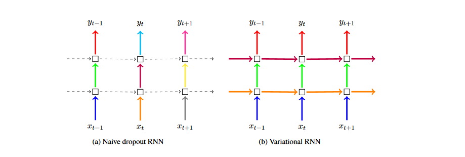
The idea here is nicely illustrated by the below figure taken from Gal & Ghahramani’s paper. The core takeaway that it is trying to get across is that we are applying the same dropout masks to the respective weight matrices at each time step rather than randomly sampling a new mask at each step.