Basic MCMC Pt. 2: The Metropolis-Hastings Algorithm

In machine learning, we often face computations over random variables that are analytically intractable and are hence forced to use Monte Carlo (MC) approximations. However, using MC approximations is only possible if we have actually have samples from the distribution of interest, something which is often not the case. In this post I will outline the idea of “Markov Chain Monte Carlo” (MCMC) methods that allow us to compute Monte Carlo approximations in such settings. Specifically, I will focus on the most basic MCMC algorithm - the Metropolis-Hastings algorithm.

Motivation

We often want to perform computations such as computing expectations of the form:

\[I = \mathbb{E}_{X \sim p}[f(X)] = \int{f(x)p(x)dx}\]

As mentioned, if we can easily sample from the distribution \(p(x)\) we can easily approximate such computations through the use of MC approximations of the form:

\[\hat{I}=\frac{1}T\sum_{t=1}^Tf(X_T), \text{where }X_1,…,X_T \sim \pi\]

Such approximations are provably unbiased and consistent estimators and will converge to the true quantity of interest as \(N\) becomes arbitarily large.

However, this obviously assumes we can easily generate samples \(X_1,…,X_T \sim \pi\) which often isn’t trivially the case. For instance, in Bayesian ML we will often run up against distributions \(\pi\) which are known only up to a normalising constant. When the distribution \(\pi\) is intractable in this sense, we cannot rely on standard sampling procedures (e.g. inverse transform sampling with a known CDF) to generate the samples we need in order to construct MC approximations.

It is in this kind of setting where MCMC comes in. MCMC methods work by constructing a chain of samples \({X_1,…X_T}\) (called a “Markov chain” for reasons outlined below) that will converge towards being samples from the distribution of interest \(\pi\) as the length of the chain \(T\) goes to infinity. We can then use these samples to evaluate the MC approximation.

Markov Chains

So, what is this Markov chain \({X_1,…X_T}\) and how can we be sure that it will tend towards being samples from the distribution of interest if we cannot directly sample from said distribution? Well, A Markov chain is a series of sequential samples where the next sample depends on the previous sample and the previous sample alone. This is known as the chain satisfying the first order Markov property.

The chain is then constructed using a Markov transition kernel. This is a function that governs where the next position of the chain \(X_{t}\) will be give the previous position \(X_{t-1}=x_{t-1}\). Specifically, it functions as a probability measure that governs the probability that the chain will end up in any region (i.e. the probability that \(X_t \in A\)) over the domain given its current position \(X_{t-1}=x_{t-1}\). So, the transition kernel is a function of the following form:

\[\mathcal{P}(x, A) = \mathbb{P}(X_t \in A|X_{t-1}=x)\]

To be precise, the transition kernel is a measurable function in its first argument and a probability measure over the corresponding probability space in its second argument. We then draw samples at each timestep according to this kernel such that the:

Importantly, we can choose how to construct the transition kernel such that if we keep drawing samples according to it we will eventually end up drawing samples from a distribution of choice. The Metropolis-Hastings (MH) algorithm is, at its core, really just a clever choice for this kernel such that we can ~magically~ draw samples from a distribution that we might not fully know. In the next section I will outline how the MH algorithm designs the kernel to do this, but feel free to skip straight to the following section since the construction itself is maybe not massively illustrative.

Constructing the MH Transition Kernel

The aim here, then, is to construct a transition kernel such that if we repeatedly sample according to it we will end up sampling from the distribution \(\pi\) that we care about. This is where a nice property of Markov chains comes in - Markov chains (under certain conditions) have “stationary distributions” which are distributions that the chains will converge to in the sense that running the chain for arbitrarily long will results in the samples being distributed according to the stationary distribution.

A sufficient condition for \(\pi\) being a stationary distribution for the chain created by the kernel \(\mathcal{P}\) is that it satisfies the following equation:

\[\int_A{\mathcal{P}(x, B)\pi(x)dx}=\int_B{\mathcal{P}(x, A)\pi(x)dx}\]

This is called the Detailed Balance Equation and states that the probability of observing a transition from a region A of the domain to a region B should be the same as observing the reverse transition if we assume we begin by sampling from \(\pi\). Thus, we want to construct a kernel to satisfy the Detailed Balance Equation, since this guarantees that the chain will eventually converge to \(\pi\).

Now, consider the following transition kernel:

\[\mathcal{P}_{MH}(x, A) = r(x) \delta_x(A) + \int_A{p(x,y)dy}\]

where \(r(x)=1-\int{p(x,y)dy}\) is the probability that the chain remains at its current position \(x\) and \(p(x, y)\) is a density that generates proposed moves of the chain. Given that the Markov chain is at some position \(x\) this kernel corresponds to proposing that the new position of the chain be \(y\) (drawn according to the density \(p(x, y)\)) and rejecting the move and remaining at \(x\) with probability \(r(x)\). We will hence call the density \(p(x, y)\) the proposal density since, at each step of the chain, we will propose the next step of the chain by drawing from this density. For instance, a common choice is to set \(p(x, y)=N(y;x,1)\).

It turns out that if the density \(p(x, y)\) satisfies the following reversibility equation

\[\pi(x)p(x, y) = \pi(y)p(y,x)\]

then \(\mathcal{P}_{MH}\) satisfies detailed balance w.r.t \(\pi\) and \(\pi\) will be the stationary distribution of the associated Markov chain! This means we similarly need to ensure that transitioning from \(x\) to \(y\) when initially sampling from \(\pi\) is just as likely as transitioning from \(y\) to \(x\) when initially sampling from \(\pi\).

However, we now face a problem, since any arbitrary proposal isn’t going to satisfy this requirement for all moves between \(x\) and \(y\). For instance, given that our chain will be proposing moves according to the target density, we will often be making moves into regions of higher probability that are more likely than the reverse moves. To ensure that we satisyf the requirement, we can introduce a scaling probability factor \(\alpha(x,y)\) that controls the probability with which we accept proposed moves. We then let our our proposed density be \(q(x, y) = p(x, y)\alpha(x,y)\) such that we draw proposed moves from \(p\) and then accept then with probability \(\alpha\).

The point of this scaling factor is to reduce the chances of making a move in the more likely direction and improve the chances of making a move in the less likely direction. In this way, the chain should become reversible, we should satisfy detailed balance, and we should converge to the target distribution \(\pi\). Thus, we want:

\[\pi(x)\alpha(x,y)p(x, y) = \pi(y)\alpha(y,x)p(y,x)\]

Let’s assume that in general we are more likely to observe transitions from \(x\) to \(y\) so that \(\pi(x)p(x, y) > \pi(y)p(y,x)\). We then say we want to accept all proposed moves from \(y\) to \(x\) (so that we set \(\alpha(y,x)=1\)). Plugging this in and re-arranging, we get:

\[\alpha(x,y) = \frac{\pi(y)p(y,x)}{\pi(x)p(x, y)}\]

for the proposed move. This fraction is sometimes called the “Hastings ratio”. However, since we want this to hold for all moves and want to use it as a probability to limit the number of overly-likely moves we accept, we need to cap this at 1. Thus, we set:

\[\alpha(x,y) = min(1, \frac{\pi(y)p(y,x)}{\pi(x)p(x, y)})\]

With \(\alpha\) set like this, the new proposal density \(q(x, y) = p(x, y)\alpha(x,y)\) satisfies the reversibility requirement. If we sub this into \(\mathcal{P}_{MH}\) we hence get a transition kernel that will target our distribution \(\pi\) as a stationary distribution! So, our transition kernel is:

\[\mathcal{P}_{MH}(x, A) = r(x) \delta_x(A) + \int_A{ p(x, y)\alpha(x,y)dy}\]

with \(r(x)=1-\int{p(x, y)\alpha(x,y)dy}\).

Crucially, the form of \(\alpha\) allows us to sample from \(\pi\) without being able to completely able to specify it. This is because if we can write

\[\pi(x)=\frac{\phi(x)}{\int{\phi(x)}dx}\]

\(\alpha\) becomes:

\[\alpha(x,y) = min(1, \frac{\phi(y)p(y,x)}{\phi(x)p(x, y)})\]

such that running this chain only requires knowing the distribution up to a normalising constant (which is something we often do know in Bayesian ML etc.). Furthermore, if we choose \(p\) to be symmetric such that \(p(x,y)=p(y,x)\), \(\alpha\) simplifies even further to become:

\[\alpha(x,y) = min(1, \frac{\phi(y)}{\phi(x)})\]

The Metropolis-Hastings Algorithm

So, what does the above construction of the MH transition kernel actually mean for the construction of an algorithm? Well, it gives us the following algorithm known as the Metropolis-Hastings algorithm to sample from some distribution of interest \(\pi\):

First, initialise the value of the chain \(x_t\) to be some arbitrary \(x_0\) and initialise the chain to be an empty list C
Then, for t = 1, …, T, do:
- Sample a proposed move for the chain: \(y_t \sim p(x_t, y_t)\)
- Sample a gating variable: \(u_t \sim U[0,1]\)
- If \(u_t < \alpha(x_t, y_t)\), do:
  - Set \(x_t = y_t\)
- Append \(x_t\) to the chain C
Return the chain C

where (assuming that the distribution we wish to sample from can be written as \(\pi(x) \propto \phi(x)\) and our proposal density is symmetric such that \(p(x,y)=p(y,x)\)) we have the acceptance probability given by:

\[\alpha(x,y) = min(1, \frac{\phi(y)}{\phi(x)})\]

Running this algorithm leads to a Markov chain of samples corresponding to the Markov chain produced using the transition kernel \(\mathcal{P}_{MH}\) described above. Since this kernel is in detailed balance w.r.t. the distribution \(\pi\), this chain will, as we run the chain for an infinite amount of time, converge to samples drawn from \(\pi\)! So, we have an algorithm that allows us to sample from \(\pi\) even if we only know it up to some normalising constant.

The Gaussian Random Walk MH Algorithm

A comman instantiation of this algorithm is to set the proposal density to be a Gaussian centered at the current value of the chain:

\[p(x,y) = N(x; y, \sigma^2)\]

This is used due to its symmetry and due to the fact that the \(\sigma\) parameter functions as a fairly standard (quasi) stepsize parameter that allows us to control how close we want successive proposed moves of the chain to be. Using this choice of proposal, the Python code for the MH algorithm (i.e. the “Gaussian random walk Metropolis-Hastings algorithm”, or, GRW-MH) is shown below.

def grw_metropolis_hastings_1D(target_density, x0, n_iters, sigma):
    xt = x0
    chain = []
    for t in range(n_iters):
        yt = xt + np.random.normal(loc=0, scale=sigma)
        hastings_ratio = target_density(yt) / target_density(xt)
        alpha = min(hastings_ratio, 1)
        u = np.random.uniform(low=0, high=1)
        if u < alpha:
            xt = yt
        chain.append(xt)
    return chain

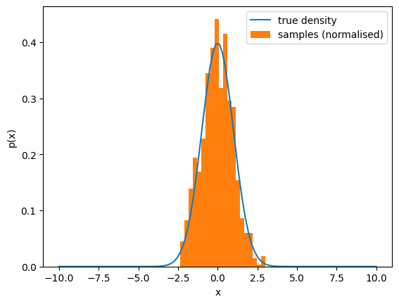
This is a very popular and powerful algorithm. To give an example of how it works, suppose we want to use it to draw samples from a standard Gaussian. The below figure shows the true density for the standard Gaussian and the (normalised) empirical distribution of samples from running the GRW-MH algorithm for 1000 iterations and intialising the chain at 0. Clearly, the chain has succesfully approximated the distribution.

Having outlined the algorithm, we can now turn attention to some practical considerations we face when actually running this algorithm.

Chain Length

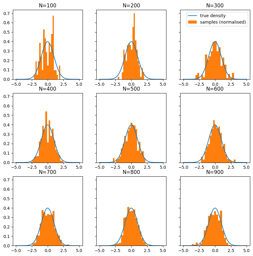
The first factor to consider when running a MH algorithm is the length of the chain. While the MH algorithm guarantees that the chain will eventually converge to the distribution we care about, it may not do so quickly. This can motivate the use of other algorithms in practice (i.e. if the MH algorithm would only converge in the infinite limit), but the key takeaway here is that if the chain converges in a sensible amount of time, its approximation to the true distribution will improve as we run it for longer.

This is illustrated in the figure below where I plot the true distribution (here, a standard Gaussian at 0) relative to the empirical distributions generated by chains of different lengths. Clearly, as we run the chain for longer, the approximation to the distribution improves. This matters since it means any MC estimates we compute with the chain will suffer from less approximation error.

Step Size

Another key consideration is step size. The step size of the chain controls how far or close proposed moves of the chain are to the current value. With the GRW-MH algorithm (i.e. MH using a Gaussian proposal) the step size is just controlled by the \(\sigma\) parameters - a larger \(\sigma\) means we will, on average, propose larger steps while a smaller \(\sigma\) means the reverse.

I have plotted the empirical distributions from the chains generated by the GRW-MH algorithm for different \(\sigma\) below (where we again target the standard Gaussian and the chain is run for 250 iterations).

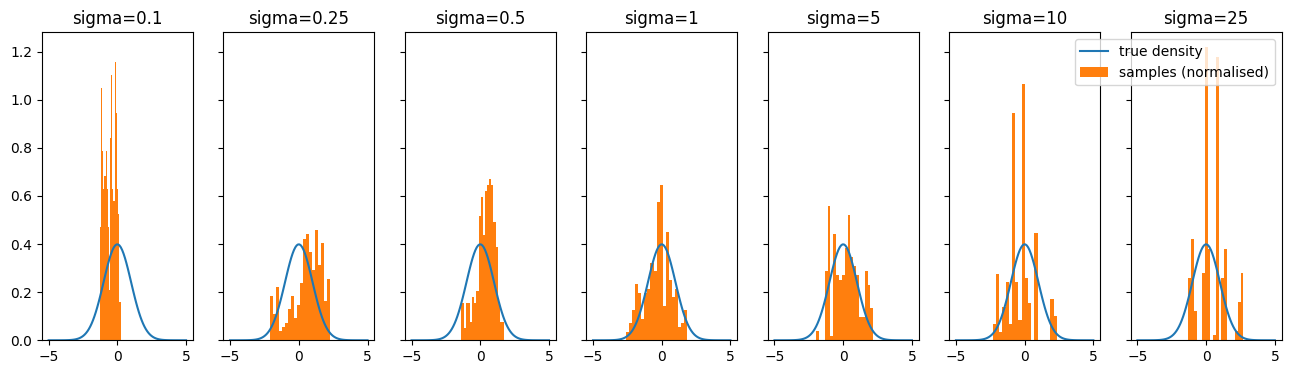
Clearly, the approximation worsens for both overly small \(\sigma\) and overly large \(\sigma\).

The approximations worsens for overly small \(\sigma\) since this corresponds to each step in the chain being very close to the prior steps. This means the chain takes way longer to explore the whole distribution and so our empirical samples will be concentrated in the regions of the domain that the chain has focused on taking small steps around.

A large \(\sigma\) causes the approximation to worsen since this corresponds to taking huge steps which will often end up being in regions of low density ; this means the Hastings ratio will often be very low and so most steps will be rejected. This then means that the chain will be “sticky” and remain at the same place for many steps. This means it will not generate a diverse array of samples from the desired distribution, leading to a poor empirical approximation. This will then lead to worse MC estimates.

Burn-In

When running the MH algorithm we also have to consider that we might be initialising the chain somewhere far away from the regions of high density under the target distribution. If this is the case, the beginning samples will NOT be drawn from the distribution that we care about as they will merely represent steps taken by the chain on its way towards the distribution we care about. We hence ought to discard these samples as they are not representative of our target distribution. This discarding of the first samples is called “burn-in” in MCMC algorithms.

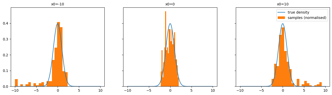
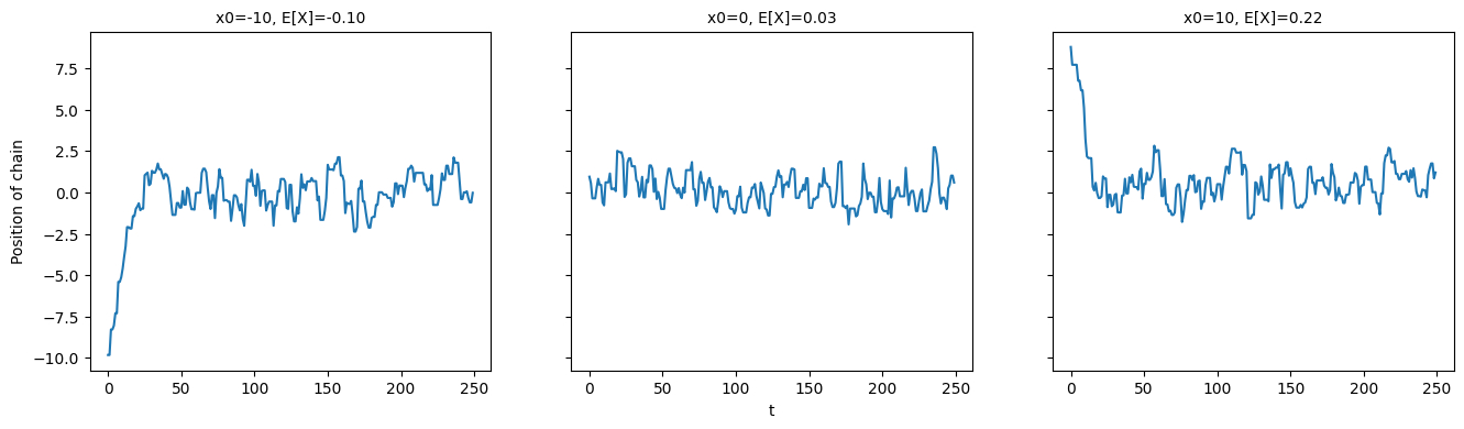
To illustrate the need to track burn-in, I ran the GRW-MH algorithm for 250 iterations to again target the standard Gaussian. However, I initialised the chain at 0, 10 and -10 to show that when we initialise far outside regions of high density (i.e. 10 and -10) we end up with some samples that are clearly not drawn from the distribution we care about and hence worsen our empirical approximation to this distribution. This is shown in the figure below, with there clearly being samples that are drawn while the chain is converging to the distribution of interest.

How can we track burn-in? Well, we can create traceplots of the variables we are running the chain over (or, in the multivariate case we can create traceplots for summary statistics). A traceplot just tracks the value of a variable at each iteration. I created traceplots to track the the three chains described above and these are shown below. These traceplots clearly show that the chains initialised far from the target distribution exhibit burn-in as they move towards the target. I have also included the MC estimates correspond to the three chains. Clearly, the two chains that have a long burn-in time produce worse MC estimates (since the true mean of the distribution is 0).

Finally, let’s consider a problem with the MH algorithm as presented. Namely, let’s consider the fact that the vanilla MH algorithm struggles with multimodal target distributions.

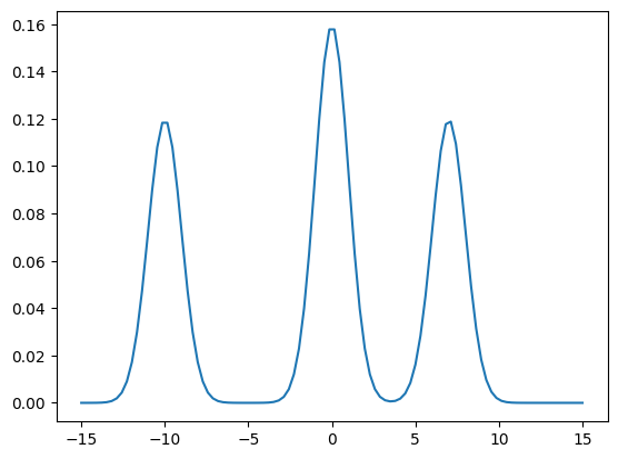
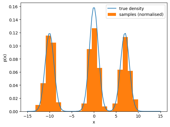
Imagine our target distribution is the following Gaussian mixture model:

\[\pi(x) = 0.4N(x;0,1) + 0.3N(x;7, 1) + 0.3N(x; -10,1)\]

This distribution is characterised by having multiple modes separated by sizable regions of negligible density as show by the plot of its density below:

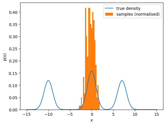
The GRW-MH algorithm faces a problem here: in order for the chain to moves between the different regions of high density, it needs to step through the regions of low density. However, the Hastings ratio for any proposed step into a region of low density will be very small such that the vast majority of these needed proposed steps will be rejected. This means that the chain will be stuck in one region of high density until it is lucky enough to get a move to one of the other regions (through a low density region) accepted.

To illustrate this effect, I ran the GRW-MH algorithm for 250 iterations (initialised at \(x_0=0\) with \(\sigma=1\)) to target this multimodal distribution. The resulting empirical distribution is shown below, and clearly illustrates that we have failed to move from the central region of high density to the other two regions.

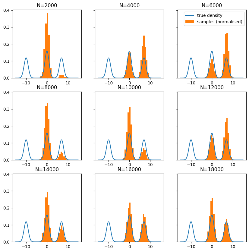
Now, if we run the chain for longer we end up being able to eventually move over to the “nearer” mode centered at 7. However, even if we run the chain for a very long time, we seem unlikely to ever get to the further mode (centered at -10). This is because getting to the further mode requires many repeated steps that are likely to be rejected while getting to the closer mode only requires a few such steps. This effect is illustrated below as I have plotted the empirical distributions of chains run for different amounts of time:

So, what can we do to overcome this problem? Well, a partial solution is to increase \(\sigma\) such that it is very large. This reduces the number of unlikely steps required to move between regions of high density, making such moves far more likely. However, doing this is problematic since a large \(\sigma\) will, as explained above, still lead to many proposed moves getting rejected (e.g. when the chain tries to step beyond the modes).

A better solution is to use a mixture transition kernel. The idea here is that if we select two transition kernels \(\mathcal{P}_A\) and \(\mathcal{P}_B\)that both have our target distribution as their stationary distribution, then linearly interpolating between then will yield another transition kernel that also has our target as the stationary distribution. That is, for \(\gamma \in [0,1]\), the kernel

\[\mathcal{P} = \gamma \mathcal{P}_A + (1-\gamma) \mathcal{P}_B\]

will be a valid MH transition kernel that will target out desired distribution!.

In practice, using this kernel leads to a MH implementation where our proposal distribution is just the corresponding linear interpolation between the two proposal distributions corresponding to the two densities. The modified mixture GRW-MH algorithm is shown below in Python:

def mixture_grw_metropolis_hastings_1D(target_density, x0, n_iters, sigma_low, sigma_high, mixture_weight):
    xt = x0
    chain = []
    for t in range(n_iters):
        yt = xt + mixture_weight * np.random.normal(loc=0, scale=sigma_low) + (1 - mixture_weight) * np.random.normal(loc=0, scale=sigma_high)
        hastings_ratio = target_density(yt) / target_density(xt)
        alpha = min(hastings_ratio, 1)
        u = np.random.uniform(low=0, high=1)
        if u < alpha:
            xt = yt
        chain.append(xt)
    return chain

This algorithm is then nice since we can get the benefits of having a large \(\sigma\) (e.g. being able to freely move between modes) without incurring all of the costs (e.g. many moves being rejected and the chain being sticky) by mixing between a proposal Gaussian with a low variance and a proposal Gaussian with a high variance.

To illustrate this, I ran this modified algorithm for 2000 iterations with the \(\sigma\) set to 1 for the low-variance Gaussian anf 5 for the high variance Gaussian. The resulting empirical distribution is shown below and clearly illustrates that this modified algorithm can better explore multi-modal distributions.

Summary

In this blog post I have outlined the msot simple MCMC algorithm (the MH algorithm) and detailed some pratical concerns that come up when using it (e.g. step size, burn-in and mutlimodality). While this has been considered in the simple uni-dimensional setting, these ideas can easily be scaled up to more complex settings. Indeed, with some minor modifications the MH algorithm can be defined for infinite dimensional spaces such that that we can perform MCMC in Hilbert spaces. This then lets us get Markov chains of (approximations to) infinite-dimensional objects like functions which is pretty cool. The idea of generating Markov chains is also crucial to advances in modern ML such as in diffusion models.