Bandit Algorithms (& The Exploration-Exploitation Tradeoff)
RL problems are unique in that RL agents face much greater uncertainty (e.g. about rewards, the environment) than is faced by models in supervised learning. This gives rise to many problems, one of which is that RL agents are forced to confront the so-called “exploration-exploitation tradeoff”. In this post, I will explore this tradeoff in the simplified context of multi-armed bandit problems. Specifically, I will investigate how different algorithms navigate this tradeoff in this setting. I will also provide the code for these algorithms so that anyone interested can play about with them further.
Note (24/08/2024): It should be noted that this blog post is one of the posts I copied over from my old blog. As such, it is a pretty word explanation of some faily simple ideas. However, I decided to copy this post over to my new blog (despite viewing it as being a fairly crappy post) since these ideas - like value functions, UCB exploration and policy gradient algorithms - are really important in understanding RL, and exploring them in the context of multi-armed bandits seems like a simple way to grok some of the core insights.
Multi-Armed Bandits
In RL, we think of an agent that is interacting with an environment. At each timestep, the agent takes some action that influences the environment and then recieves some reward. The overall aim of the agent is to maximise its return, or the (discounted) sum of its rewards. Crucially, the agent does not know its reward function and hence has to perform actions and see what rewards it gets in order to make inferences about what kinds of actions provide it with high rewards.
The agent hence faces a tradeoff - it can either keep performing the actions that it already knows provide it with high rewards, or it can choose to perform actions for which it is uncertain what the reward will be. The idea here is that the agent may “know” that some actions will lead to a good reward but may have some other actions for which it is highly uncertain what the return would be. Such uncertain actions could, then, potentially lead to massive long-run returns. Hence, the agent faces the so-called “exploration-exploitation tradeoff”, since it must balance exploiting the actions it knows will yield a good reward and exploring new actions which could possible yield an even better reward.
Now, this explanation is a bit simplistic relative to how RL actually works. This is because RL agents can take actions that end up influencing their environments, such that they have to overcome problems like building models of the environment and so on. These topics are really cool, but we can simplify the setting to focus in on the exploration-exploitation tradeoff. We can do this by focusing in on multi-armed bandit problems.
Multi-armed bandit settings are settings where the environment only has a single state. This makes RL way easier, since it means agents can ignore the effect of the actions thet take on the environment. In a bandit setting, agents must choose which of a set of actions to perform at each timestep. They will then recieve a (random) reward associated with the action they performed. Thus, the environment in this setting is just:
\[E=\{ p(r|a) | a \in \mathcal{A}\}\]
where \(\mathcal{A}\) is the set of possible actions the agent can perform and \(p(r|a)\) are the distributions of rewards associated with the agent performing action \(a\).
Importantly, the “problem” we face in bandit setting is that the agent does not know what the distributions of rewards are. Thus, it has to have some strategy for exploring actions and then performing those that yield a high reward. This means we face having to trade off exploring different arms whilst exploiting our knowledge of arms that we know to be “good”. We can think of this as sitting on a casino floor surrounded by slot machines. Each machine has an arm which we can pull and each machine has its own distribution of rewards. Our goal, then, is to come up with some plan for winning money from these machines.
A Toy Bandit Problem
There are many different algorithms - which I am refering to as “bandit algorithms” - to guide an agent in this setting. I will explore three basic such algorithms in the context of a toy problem. Specifically, I will use a bandit problem where an agent has 11 actions to choose from. The reward distributions of these 11 actions are merely shifted standard Gaussian centered at the integers from -5 to 5. So, our “actions” are basically picking one of these 11 integers such that \(\mathcal{A} = \{-5,4,…,4,5\} \) and our “environment” is merely:
\[E=\{ \mathcal{N}(a, 1) | a \in \mathcal{A} \}\]
Clearly, the optimal action in this toy set-up is to merely keep pulling the final arm (i.e. the one corresponding to +5). However, our agents do not know this and so our algorithms need to let them act in some way as to “figure it out”. The goal of the algorithms I consider is hence to learn a policy \(\pi(a)\)- a distribution over actions - that achieves a high reward over the long run.
Action-Value Estimates
The first three algorithms I will consider all work by estimating the expected value of each actions. The idea here is that the rewards associated with each action have some true expected value. Call this \(q(a)\). If the agent new these rewards, the problem would be trivial as the agent could merely just keep performing the action with the highest expected reward. However, in practice, \(q(a)\) is unkown to the agent. These first three algorithms - which we can call action-value algorithms - work by building some estimate \(Q_{t}(a)\) of the true expected value for each action at each time step. They then use these estimates to decide how to act. The t subscript here is important since these estimates will change over time.
So, how do agents build these action value estimates? Well, in the simplest case we can merely let the estimated value for action a at time t be equal to the sample average reward recieved whenever the agent performed action a at any time up to time t. Using indicator functions, we can write this as :
\[Q_{t}(a)=\frac{1}{N_{t}(a)}\sum_{i=0}^t\unicode{x1D7D9}(A_i=a)R_i, \text{where } N_{t}(a)=\sum_{i=0}^t\unicode{x1D7D9}(A_i=a)\]
where \(A_i \in \mathcal{A}\) denotes the action taken at timestep \(i\) and \(R_i \sim p(r|A_i)\) is a reward drawn from the associated reward distribution. However, calculating expected rewards using the above requires us to store the entire history of actions and rewards. While possible in a toy problem like this, such a requirement is clearly infeasible for actual problems. Thus, we can update action value counts and estimates in an online fashion by updating the estimate for the action \(A_t\) performed at each time step as shown below:
\[Q_{t}(A_t)=\frac{N_{t-1}(A_{t-1})Q_{t-1}(A_t) + R_t}{N_{t-1}(A_t)+1}\] \[N_t(A_t) = N_{t-1}(A_t) + 1\]
and leaving all other estimates unchanged.
With this outlined, we can now turn to the specific algorithms and how they approach the tradeoff between exploration and exploitation. All the algorithms have a common form of choosing some action, recieiving a reward and then (optionally) updating action value estimates. As such, I use the following wrapper for all the algorithms:
class BanditAlgorithm:

    def __init__(self, algorithm, reward_dists):
        self.arm_value_estimates = {arm: 0 for arm in reward_dists}
        self.arm_counts = {arm: 0 for arm in reward_dists}
        self.reward_dists = reward_dists
        self.algorithm = algorithm

    def __call__(self, n_steps):
        actions = []
        rewards = []
        for step in range(n_steps):

            # policy - choose arm to pull and get reward
            action, reward = self.algorithm(self.arm_value_estimates, self.arm_counts, self.reward_dists)

            # perform updates
            self.arm_value_estimates[action] = (self.arm_counts[action] * self.arm_value_estimates[action] + reward) / (self.arm_counts[action] + 1)
            self.arm_counts[action] += 1

            # track actions and rewards
            actions.append(action)
            rewards.append(reward)

        return actions, rewards
Greedy Algorithm
The simplest possible algorithm in the face of the bandit problem is to merely adopt a greedy policy. Adopting such a policy merely means selecting the action with the highest value estimate at each timestep. Thus, the greedy policy is merely:
\[ \pi_t(a) = \begin{cases} 1 &\text{if } a = argmax_bQ_t(b)\\\
0 &\text{otherwise} \end{cases} \]
In Python, we can implement this as follows:
class Greedy:
    def __call__(self, arm_value_estimates, arm_counts, reward_dists):
        action_idx = np.array(list(arm_value_estimates.values())).argmax()
        action = list(arm_value_estimates.keys())[action_idx]
        reward = reward_dists[action]()
        return action, reward
On the face of it, this might seem like a sensible course of action - if we believe some action to be more rewarding in expectation, it perhaps makes sense to perform it. However, in practice this is a pretty terrible strategy since it corresponds to putting full weight on the exploitation side of the exploration-exploitation tradeoff. As such, it means that our agent may never perform many actions that have huge return. This is because the moment the estimate value for an action exceeds the value at which estimated values are initialised the greedy algorithm will just keep repeating that same action and may never even try other actions with a higher reward.
In our toy bandit setup, we initialised all value estimates to zero. Thus, once an action achieves a higher estimated value than 0, the agent will just keep performing that action and may nevery get a chance to explore other actions at all. Since I have configured the algorithm in such a way as to perform the action corresponding to the lowest integer when there is a tie, this means that the greedy policy will explore actions only until it arrives at action 1 at which point it will (in all probability) keep performing that action ad infinitum. The rewards achieved by this algorithm for 250 timesteps are shown below, and the behaviour is clearly illustrated (e.g. the rewards are clealy draws from a Gaussian at 1 after a certain number of steps).
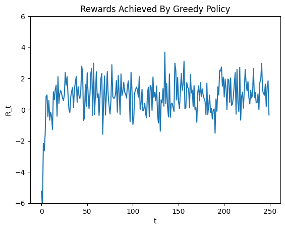
This, though, is clearly sub-optimal since we know that the best action the agent can do is to recieve rewards from the Gaussian centered at 5 instead. What has gone wrong here is that the greedy policy is merely exploiting what it knows to be a good action and fails to explore sufficiently. This means it fails to realise that there are other actions that have higher possible returns.
Now, of course, the “failure” of the greedy approach here follows from the fact that we initialised our value estimates to zero. So, one could argue that the algorithm would work well if we were merely incredibly optimistic with our initial value estimates (say, initialising all values as 1000). This is because such an initialisation would encourage the agent to explore all actions since all actions would seem inferior to its prior expectations. However, this is not a scalable approach. This is mainly because it relies on the assumption that we know the rough range in which rewards will fall, which is a pretty unrealistic assumption in many cases. It is also an incredibly ad-hoc solution that doesn’t get to the core of the failure here - that the algorithm seems to put too much weight on exploitation over exploration.
Epsilon Greedy Algorithm
So, the problem with the above greedy approach was that it relied too much on exploiting its knowledge of what it considered good actions and hence failed to explore actions which it hadn’t tried but that might have been better. Basically, we can see the above failure mode as the agent commiting to exploit one action which seems “okay” despite being very uncertain about the values of other actions. Intuitively, we want an agent to reduce the uncertainty about the rewards of all actions to at least a cetain extent so that we are justified in believing that there are not huge unrealised gains from actions we haven’t explored sufficiently.
This, then, motivates the epsilon greedy algorithm. This algorithm is very similar to the simple greedy approch but introduces a parameter \(\epsilon\). This then leads to a policy whereby, with probability \(\epsilon\), the agents selects some action at random and, with probability \(1-\epsilon\) the agent selects the action with the highest estimated value. The epsilon-greedy policy is hence given by:
\[ \pi_t(a) = \begin{cases} 1-\epsilon + \frac{1}{|\mathcal{A}|}\epsilon &\text{if } a = argmax_bQ_t(b)\\\
\frac{1}{|\mathcal{A}|}\epsilon &\text{otherwise} \end{cases} \]
and my Python implementation is given by:
class EpsilonGreedy:
    def __init__(self, eps):
        self.eps = eps
    def __call__(self, arm_value_estimates, arm_counts, reward_dists):
        if np.random.rand() < self.eps:
            action = list(arm_value_estimates.keys())[np.random.randint(0, len(arm_value_estimates.keys()))]
        else:
            action_idx = np.array(list(arm_value_estimates.values())).argmax()
            action = list(arm_value_estimates.keys())[action_idx]
        reward = reward_dists[action]()
        return action, reward
The intuition underlying this algorithm is that we are just trying to create a form of the greedy algorithm that properly explores the entire space of actions and hence reduces sufficiently uncertainty about action rewards. This policy does this by sometimes selecting a random policy. This should lead to better estimates of all action values and should, hence, not miss out on actions with high expected rewards.
The below figure illustrates the rewards achieved by the algorithm over 500 iterations for 3 different values of epsilon (0.001, 0.01 and 0.1).
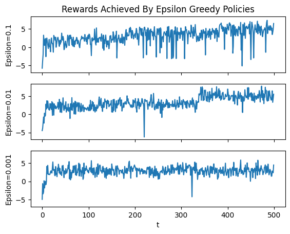
Clearly, this is an improvement over the simple greedy approach for all epsilon. However, it is also clear that the largest epsilon manages to converge to recieving rewards from the optimal distributon fairly quickly while the middle epsilon takes longer and the smallest epsilon fails to achieve this at all over the 500 runs. What is happening here is that epsilon controls how much we trade off exploration for exploitation - a larger epsilon means we place more weight on exploring and less on exploiting our knowledge of what we think is a good action.
However, a large epsilon has its drawbacks as shown by the graph for the 0.1 case. This is because, even once the agent has sufficiently explored the environment to find the best action, it keeps exploring at the same rate. This is because epsilon is constant and hence every 10th action will, on average, be random even once we know what actions are good and what actions are bad. This means we can improve further on the epsilon greedy algorithm.
Upper Confidence Bounds
So, how can we make such an improvement? Well, the epsilon greedy approach failed since it kept exploring even after we had reduced uncertainty enough to be relatively confident about which actions had the highest action values. Thus, what we broadly want is an algorithm that explores actions a lot when our uncertainty over their values is high and then explores less and less as this uncertainty reduces.
This is sometimes called “optimism in the face of uncertainty” and represents a theoretically well-founded approach to the exploration-exploitation tradeoff. The idea here is that when we are very uncertain about the value of actions we should be optimistic and perform them. This is because they may have a high expected value and so performing them gives us a chance to investigate whether this is the case.
Optimisim in the face of uncertainty gives rise to the UCB algorithm, where UCB stands for “upper confidence bounds”. The UCB algorithm is similar to the original greedy algorithm except that, rather than being greedy with estimated values, we are greedy with respect to upper bounds on what we think these values could be. That is, we come up with some upper confidence \(U_t(a)\) for each action such that the true value \(q(a)\) is less than our upper confidence bound \(Q_t(a) + U_t(a)\) with a high probability. That is, we select \(U_t(a)\) such that with a high probability it holds that:
\[q(a) < Q_t(a) + U_t(a) \]
We then select actions to be the actions with the highest upper confidence bound:
\[a_t = argmax_{a \in \mathcal{A}}(Q_t(a) + U_t(a))\]
The intuition here is that we are selecting the action for which it is plausible that the expected value is the largest. Since large expected values will be plausible for actions which haven’t been tried much, this will encourage exploration for uncertain actions. However, unlike the epsilon greedy approach, this epxploration will reduce once we are certain of what actions are good.
So, how do we select \(U_t(a)\)? Well, it can be shown that a good choice is to set it such that:
\[U_t(a) = \sqrt{\frac{2log(t)}{N_t(a)}}\]
Why is this a good choice? Without going into too much theory its kind of hard to explain rigourously but a broad outline is as follows. We can judge bandit algorithms in terms of how the total “regret” of agent grows over time, where the regret at each timestep is the difference between the expected value of the optimal action and the expected value of the performed action. We can hence see the goal of the agent as being to minimise total regret. It turns out that regret growth for the UCB algorithm with this \(U_t(a)\) is exactly logarithmic. This is good since both the prior algorithms (and the following one I outline shortly) have linear regret growth. Additionally, it can also be shwon that regret will grow at least logarithmically. Thus the UCB with this \(U_t(a)\) leads to agents achieving the optimlal rate of regret growth.
In practice we can replace the \(\sqrt{2}\) with a parameter \(\alpha\). This still allows us to achieve our bound but having the paramter allows us to explicitly control how much we wish to trade off exploration and exploitation. A larger \(\alpha\) corresponds to placing a greater weight one exploring to equally reduce the uncertainties of all action values whilst a lower alpha corresponds to placing a greater weight on exploiting actions that are known to have good action values.
Having explained all of that, the policy provided by the UCB algorithm is then:
\[ \pi_t(a) = \begin{cases} 1 &\text{if } a = argmax_{b \in \mathcal{A}}(Q_t(b) + \alpha \sqrt{\frac{log(t)}{N_t(b)}})\\\
0 &\text{otherwise} \end{cases} \]
and my Python implementation is:
class UCB:
    def __init__(self, alpha):
        self.alpha = alpha
    def __call__(self, arm_value_estimates, arm_counts, reward_dists):
        t = np.sum(arm_counts.values())
        ns = np.array(list(arm_counts.values()))
        ns = np.where(ns == 0, 0.01, ns)
        us = (1 / (2 * ns))
        upper_bounds = np.array(list(arm_value_estimates.values())) + self.alpha * us ** 0.5
        action_idx = upper_bounds.argmax()
        action = list(arm_value_estimates.keys())[action_idx]
        reward = reward_dists[action]()
        return action, reward
To illustrate the performance of UCB, I ran the algorithm with \(\alpha = \sqrt{2}\) for 500 steps and have displayed the resulting rewards at each iteration in the graph below.
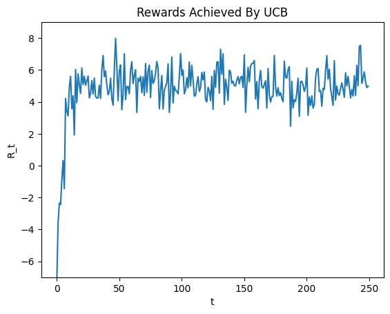
Clearly, we get good results with the algorithm. Not only do we rapidly converge to the optimal action, but we also keep recieving rewards drawn from the optimal distribution rather than keeping exploring sub-optimal actions for too long.
Comparing Action-Value Algorithms
We have hence considered an array of different action value algorithms that all work in various ways by estimating the action value of the different actions \(a \in \mathcal{A}\). To illustrate how these algorithms differ in performances, I ran all algorithms again for 1000 iterations, 1000 times over (e.g. I ran each algorithm for 1000 steps 1000 seperate times) and averaged the rewards each algorithm achieved at each timestep. Running the algorithms 1000 times over and averaging rewards should reduce sampling variability and better allow us to inspect the trends. The results are shown in the figure below.
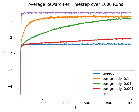
From this figure we can see all of the theoretical points explained above:
- The plain greedy algorithm is just bad - it leans too far on the exploit side of the explore-exploit tradeoff and doesn’t realise there are actions with higher possible values
- The epsilon greedy algorithm is okay, but we face a tradeoff in setting the \(\epsilon\) parameters. For large \(\epsilon\) rewards increase quickly but bottom out below the optimal possible value since this corresponds to randomly exploring with a high probability even once we know what actions are good. For small \(\epsilon\) we explore slower but experience less suboptimal exploration once the optimal is reached.
- The UCB algorithm converges rapidly and strictly dominates ; this makes sense given the afforementioned theoretical guarantees we can provide.
Policy Gradient Algorithms
All of the above algorithms work by estimating action values. This corresponds to a more general strategy in broader RL of estimating value functions. An alternative strategy in RL is to parameterise the policy of an agent and then converge to an optimal policy by taking steps of gradients ascent. This is the so-called “policy gradient approach”.
In a a simple form, let us have a vector of “preferences” as follows:
\[\boldsymbol{h_t} = [h_t(a_1), …, h_t(a_k)]^T\]
where each the relative size of the preference for action \(a\), denoted \(h_t(a)\), represents how much more likely that action should be under the policy \(\pi_T\). The policy can then be viewed as a distribution over actions by passing the preferences vector through a softmax such that the policy is given by:
\[\pi_t(a|\boldsymbol{h_t}) = \frac{exp(h_t(a))}{\sum_{i=1}^k exp(h_t(a_k))}\]
The nice thing about this is that, since we have parameterised the policy with the preferences, we can update the preferences such that the expected value of the reward at the next time step increases. This is because the expected value of the reward \(\mathbb{E}[R_t|A_t=a]\) is just a function of our new paramters. We can then update like this with standard gradient ascent such that we update preferences according to:
\[\boldsymbol{h_{t+1}} = \boldsymbol{h_t} + \eta \nabla_{\boldsymbol{h_t}}\mathbb{E}[R_t|\pi_t]\]
where \(\eta\) is a standard stepsize parameter.
What then, is \(\nabla_{\boldsymbol{h_t}}\mathbb{E}[R_t|\pi_t]\)? Well, using the REINFORCE trick that is common in RL it turns out that:
\[\nabla_{\boldsymbol{h_t}}\mathbb{E}[R_t|\pi_t] = \mathbb{E}[R_t\nabla_{\boldsymbol{h_t}}log\pi_t(a|\boldsymbol{h_t})]\]
which we can approximate using a Monte Carlo approximation with a sample size of 1 at each step such that our gradient ascent update rule is:
\[\boldsymbol{h_{t+1}} = \boldsymbol{h_t} + \eta R_t \nabla_{\boldsymbol{h_t}}log(\pi_t(A_t|\boldsymbol{h_t}))\]
Using the earlier-described preference set-up (e.g. passing through a softmax to get the policy), this corresponds to the following update rule in practice:
\[ h_{t+1}(a) = \begin{cases} h_t(a) + \eta R_t(1-\pi_t(a|\boldsymbol{h_t})) &\text{if } a= A_t\\\
h_t(a) -\eta R_t\pi_t(a|\boldsymbol{h_t}) &\text{if } a \neq A_t \end{cases} \]
Intuitively, this means that whenever we select an action, we will increase the magnitude of its preference (while decreasing those for other actions such that we retain a valid PMF). Crucially, we increase the magnitude more for actions that yield larger rewards so that, eventually, the preferences for the largest rewards will dominate.
My code for this algorithm is provided below.
class PolicyGradient:
    def __init__(self, alpha, n_arms):
        self.alpha = alpha
        self.preferences = np.ones(shape=(n_arms,))
        self.probs = np.exp(self.preferences) / np.exp(self.preferences).sum()
    def __call__(self, arm_value_estimates, arm_counts, reward_dists):
        action_idx = np.random.multinomial(1, self.probs).argmax()
        action = list(arm_value_estimates.keys())[action_idx]
        reward = reward_dists[action]()
        update = -1 * self.alpha * reward * self.probs
        update[action_idx] = self.alpha * reward * (1 - self.probs[action_idx])
        self.preferences += update
        self.probs = np.exp(self.preferences) / np.exp(self.preferences).sum()
        return action, reward
To compare this to the value algorithms, I again ran it, the epsilon-greedy algorithm and the UCB algorithm for 1000 timesteps 1000 times over and averaged the rewards at each timestep for each algorithm. The results are shown in the figure below:
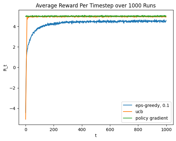
We can see that the policy gradient algorithm performs equally well as the UCB algorithm. This is a kind of cool result since the policy gradient approach handles the exploration-exploitation tradeoff automatically, without us having to hard-code it in!
Summary
In this post, I have outlined how various algorithms interact with the need to tradeoff exploring vs exploiting in the simplified RL setting of multi-armed bandits. This is, I think, a pretty interesting topic, especially when we scale up to full RL problems where actions impact environment states. A notebook I made corresponding to this post can be found here if anyone wants to play around with the algorithms further.
Enjoy Reading This Article?
Here are some more articles you might like to read next: